Google Sheets techniques (Episode 2)
Contents
- Contents
- Introduction
- Challenges of array formulas
- Components of Map tab
- The Map tab as a “Map” of the data
- Why split the Inventory into two tabs?
- Wow, it seems like a lot of work. Is it worth it?
- How to build upon the template
- Conclusion
Introduction
In our previous episode, we covered some techniques to improve performance and readability for Google Sheets that contain a lot of formulas. One of those techniques was the use of array formulas. However, array formulas do come with their own constraints to manage, and this episode will cover a solution to manage them: the Map tab. Feel free to make a copy the sample use case we’ll be covering from here.
In our example use case, we have a spreadsheet that helps compute the total value of an inventory of fruit in local currency. TThe spreadsheet consists of several tabs.
- Inventory_Input: The data tab called that will contain data on fruits, with columns for the name of the fruits, the quantity, and the unit price of each fruit in USD
- Interface: Our user interface tab, which contains a field for users to input a currency exchange number for USD to their local currency, and an output field computing the total value of the fruit inventory in local currency. This output field computes its output based on the data in “Inventory_Input” as well as the exchange rate input from the user
- CALC_Inventory: A calculation tab which contains calculations
- MAP: The Map tab, which we will go into more detail later on
Challenges of array formulas
When using array formulas to process data, there are two main ways to refer to the columns that we are using in our computations: full column ranges (eg A:A), or bounded ranges (eg A1:A1000). Each of them have different advantages and drawbacks. Full column ranges have a higher performance overhead, but will dynamically respond to the number of rows changing. Bounded ranges have a lower performance overhead, but by default do not respond dynamically to the number of rows changing.
When we have a large spreadsheet with many formulas and columns, it’s important that performance is manageable, and that maintenance is manageable (ie we do not have to manually update many formulas each time the size of the data changes). The Map tab aims to accomplish this.
Components of Map tab
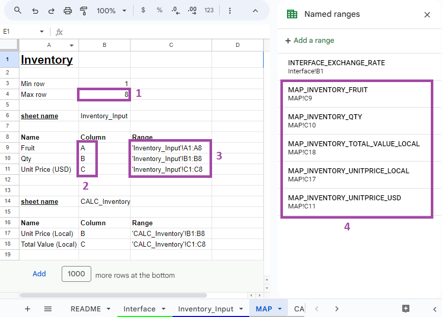
The Map tab consists of several key components.

- A row counter that counts the number of rows in a sheet
- A column checker that returns the column letter of a given column
- A string that concatenates sheet name, column, and rows to create a range string (eg Sheet1!A1:A10)
- Nameranges that refer to the ranges strings in the tab
What the map tab is doing is reducing the number of time full column ranges are called in array formulas from “every time a column is referenced” to “once per data tab”. This drastically reduces the performance overhead while retaining the benefit of dynamically responding to varying number of rows. How does it accomplish this via each of the components? Let’s step through each of them to find out.
Row counting
=ARRAYFORMULA(
    MAX(
        IF(
            LEN(Inventory_Input!A:A),
            ROW(Inventory_Input!A:A),
            )
        )
    )
This row counting formula helps to find the maximum row in the input data tab that contains data. The row number returned will then be referenced by other formulas to generate bounded range strings without having to each utilise a full column range reference.
Column checker
=REGEXEXTRACT(
    ADDRESS(
        1,
        COLUMN(Inventory_Input!A$1)
        ),
    "[A-Z]+"
    )
This formula extracts the column letter of a given column. The reason why we formularise this instead of entering a letter like “A” directly is to allow the column reference to shift left or right if we insert or delete columns. For example, if a column was inserted to to left of column A, our example reference above would start returning B instead of A. This implementation helps to reduce the maintenance needed as we expand our spreadsheet.
Creating a range string
=CONCATENATE(
    "'",
    $B$6,
    "'!",
    B9,
    $B$3,
    ":",
    B9,
    $B$4
    )
This formula concatenates the sheet name, column letter, and row numbers together into a range string that we can use in formulas. As the number of data rows or the columns change, the row counter and column checkers will update, and update this range string accordingly, allowing us the benefit of increased performance of bounded column ranges for our array formulas, while managing the downside of maintenance overhead.
Nameranges
As is good practice, we give each of our ranges a name to refer to them by. It’s much easier to understand what INDIRECT(MAP_INVENTORY_QTY) * INDIRECT(MAP_INVENTORY_UNITPRICE_LOCAL) means, compared to INDIRECT(MAP!C10) * INDIRECT(MAP!C17).
The Map tab as a “Map” of the data
The map tab contains all the range strings for all the data in the entire spreadsheet. It provides a central place to look up what data a spreadsheet contains, and where it is located. This is extremely helpful for human readability, not just for making our formulas work. If we wanted to, we could even add a “Description” column where we can describe the contents of each column and turn the Map tab into a data dictionary.
Why split the Inventory into two tabs?
The Inventory data is split across two tabs, “Inventory_Input” and “CALC_Inventory”. This is to segregate input data that comes from an external source or the user, from data that is entirely generated by formulas. With this segregation, users can feel comfortable inspecting and correcting data in data tabs, without the stress of working in a tab where some columns are data they can modify, and other columns are formulas that they have to be careful not to break.
From a data model standpoint, the two tabs can be considered the same “data frame”. They contain the same number of rows, and the n-th row in “Inventory_Input” refers to the n-th row “CALC_Inventory”. I chose to name the named ranges for columns in both these tabs with the same “MAP_INVENTORY” prefix to convey them as both being part of the Inventory table.
Wow, it seems like a lot of work. Is it worth it?
It depends. For one-off spreadsheets that take less than 15 minutes to build, and that you will almost never look at again, it’s absolutely not worth it to take this much effort to implement a map tab. However, if your spreadsheet takes more than a few hours to build, and it’s something you want to come back to to review or build upon, or you need to hand over to someone else, then it’s absolutely worth it. I’ve used these techniques in a professional setting, and it’s made onboarding new team members and allowing them to build upon existing assets much easier. It’s allowed me to come back to personal projects like the savings calculator two years after last working on it and quickly re-familiarising with it to build an updated version.
Remember, code spends 90% of its time being read, 10% of its time being written. Making that 90% easier is a huge benefit.
How to build upon the template
All this setup is to make expanding on the existing spreadsheet easier. But what exactly do you need to do to expand the spreadsheet?

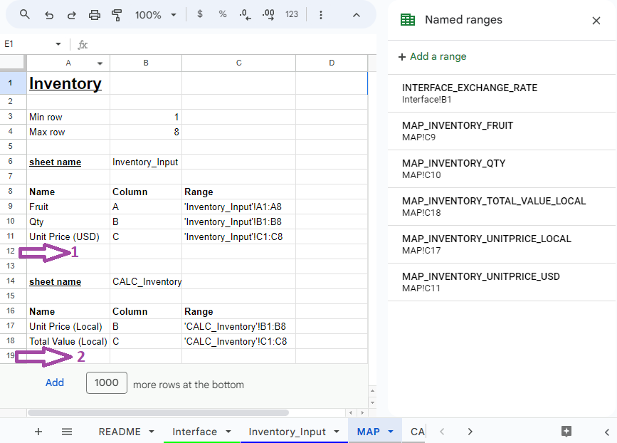
If you wanted to add more columns to the Inventory table, you would add more rows at 1 (pictured above) for data input columns, and more rows at 2 (pictured above) if you wanted to add more calculated columns.
If you wanted to add more data tables, you could copy the entire block from A1 to C18, and paste them into new rows below. Remember to update the “data table” name from “Inventory” to your new data table name, the sheet names to your new sheet names, as well as the formula references in all the pale blue cells.
Conclusion
The Map tab is a setup that can help make large spreadsheets easier to manage, AND speed them up. Spreadsheets are a powerful tool for creating number crunchers that take in user input. Keeping your spreadsheets responsive and easy to maintain will make your work more productive. Don’t forget to apply the techniques learnt here and in our previous episode!
Enjoy Reading This Article?
Here are some more articles you might like to read next: